Fundamental vs Simulation Models for Energy Portfolios

There seems to be some confusion regarding the differences between, and best uses for, fundamental and simulation models.  In part, this is the fault of the vendors, who try to sell their solution as good for everything. There is no individual model that should be used for every analytical task. 

Recently I heard a chief officer of an energy company ask why his company needs simulation-based analytics, when they already have a fundamental model?  This article is designed to answer that question.

Fundamental vs Monte Carlo Simulation models

Fundamental power system analytics are typically used to build up an analytical representation of a market (generation, transmission, load). Making assumptions about grid topology, available generation capacity, maintenance outages, weather patterns, and aggregate load, these fundamental models will compute least-cost dispatch and optimal market pricing at an hourly granularity for many years into the future.  This is no small feat and fundamental models are quite good at this. A fundamental model is best used to develop a long-term forecast of hourly prices, particularly for use to inform resource planning efforts. Of course, this “single-path“ market forecast is always wrong, but if the model assumptions and inputs are good, these models can produce useful results. 

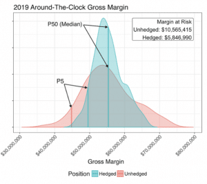
Knowing that the single-path forecast is going to be wrong in unforeseen ways, companies will turn to simulation models to understand a portfolio’s risk, or sensitivity to uncertainty, as prices deviate from the expected forecast. The simulation model will run hundreds or thousands of market simulations and probabilistically weight the results.  This yields a distribution of outcomes where the expected value is reported as well as the size, shape and magnitude of uncertainty within the distribution. Distributions can be inspected at any time granularity (hourly, monthly, annually) on metrics like portfolio gross margin, total costs, generation, fuel burn, and more. The left side of the distribution is interpreted as the “downside risk”.  Companies use the magnitude and timing of these downside risk events to hedge their portfolio and increase certainty around future cash flows. 

Fundamental models are not suited to generate robust distributions of value and therefore are inappropriate for assessing the effectiveness of existing hedging strategies or developing new ones.

Market Price Simulation

Price simulation is the key component to any simulation framework since market prices are a primary driver of risk. Different markets have very different pricing dynamics. Hourly power price shapes vary by day-of-week, month-of-year, and pricing location. Correlations between pricing locations and across commodities (e.g., between power and gas) vary seasonally. Volatility, the likelihood of price spikes, and mean reversion rates, all vary seasonally as well.  These price dynamics can strongly influence cycling behavior for thermal assets and impact both value and risk for intermittent renewable resources.

Many portfolio managers ask about fundamental drivers such as weather, grid topology, available generators, demand, etc. In most cases, these fundamental drivers are well represented in each market’s unique price dynamics, and therefore can be captured in the price simulations.

Interestingly, a commonly used integration between fundamental and simulation models involves using the forward-looking market price forecast generated by the fundamental model as input to the simulation model.  The simulation model will then produce thousands of hourly price paths around it, yielding the distributions needed for risk and hedging analysis while remaining consistent with the fundamental forecast itself.

Physical Asset Optimization & Valuation

Many years ago, energy analysts routinely used simple “closed-form spread option” models to value power plants.  Spread option models use a price for fuel and a price for electricity, as well as the volatility of each and the correlation between the two.  In a given month, if the expected spark spread was sufficient, the power plant was assumed to run.  If not, it was assumed to shut down.  Of course, this is an over-simplification of how power plants operate.  There are dozens of physical operating characteristics and costs that “constrain” the optimal operation of a power plant.  Modern dispatch models use a very detailed set of characteristics to accurately represent an asset so that modeled output is as close as possible to true asset operations.  Most simulation and fundamental models both use these modern techniques.  The difference is the simulation model dispatches assets to hundreds or thousands of hourly price paths, while still maintaining all operating constraints.  This yields hourly/daily/monthly/annual distributions of values for generation, costs, fuel burn, gross margin allowing for more effective hedge decisions. 

Other assets, such as renewables and storage, require separate analytical methodologies but still need to be integrated into a comprehensive portfolio analysis to properly track their effects on value and risk.  Renewable assets are non-dispatchable, but their hourly production can still be simulated and combined with market price simulations to develop distributions of generation and analyze the effects of volumetric uncertainty (swing risk) on asset value.  Such an analysis provides insight into production variability, price uncertainty, and even basis risk between a generation node and corresponding settlement hub.

Unlike renewables, batteries are dispatchable and their charge/discharge operations can be optimized to market prices or retail rates. Since batteries generate no electricity themselves, their value is entirely derived by operating them intelligently relative to various sources and sinks of energy at the battery site along with their corresponding values and/or costs (e.g., customer load, co-sited renewable generation, retail rates including TOU schedules and demand charges, and wholesale prices or export compensation rates).  Other asset types can and should be included in a comprehensive portfolio analysis. 

Contract valuation, Risk Management and Hedge Optimization

At a high level, we have discussed some of the differences between sophisticated fundamental and simulation models.  Using a simulation model, we generate thousands of hourly price paths that capture market dynamics and represent a very large set of possible future outcomes. These outcomes are probability-weighted and allow reporting not only on expected (mean) prices and portfolio value, but also left-tail and right-tail risk levels.  We can use these price simulations to optimize and value our physical assets, yielding many other useful statistics to support asset management and budgeting activities.  Finally, we can also use the same price simulations to value our physical and financial contracts.  These contracts can come in the form of standard swaps & options, index deals, heat-rate-call-options, revenue-put-options, PPAs, or other exotic derivatives and structured transactions.  Each of these contracts, including PPA Valuation, have unique payoff functions. 

Most importantly, we can aggregate all the above analysis based on both forward and spot price simulations to forecast distributions of portfolio cash flow through time. By bringing together all of these values, we can calculate summary statistics for the total portfolio – including both physical assets and financial contracts.  This affords the analyst / portfolio manager insight into the timing of all cash flows and how they are being generated. 

By looking at the distributions of value across months, peak periods, asset types, sub-portfolios, and many other dimensions, one can understand how, when, and why risks enter the portfolio.  This leads to the final piece of the puzzle: hedging the portfolio. 

Deciding on and implementing a hedging strategy depends on many input factors.  But armed with the analysis described above, we have all the analytical components we need to measure the risk-reduction-value (RRV) of a prospective hedging strategy.  The process above has given us distributions of value through time for every item in the energy portfolio, paving the way for effective energy portfolio optimization. This optimization accounts for the interactions between all the individual components to provide a “rolled-up” total portfolio view.  We can now assess various hedge strategies or evaluate individual contracts, assets, etc. to see the net effect they produce on the entire energy portfolio. 

No other model methodology will allow this type of analysis.  Fundamental models are very useful in their own right, but their deterministic outlook has limitations for portfolio analytics. Traders, portfolio analysts and energy risk managers should be utilizing a robust simulation-based methodology for deal valuation, cash-flow analysis, asset and hedge optimization.   

Why cQuant.io?

cQuant.io is a team of experienced PhD quants and energy analysts. cQuant develops sophisticated analytic models and delivers these solutions in a cloud-based application.  Our team has extensive experience delivering portfolio & risk analytic solutions to energy companies, including IPPs, utilities, trading floors, community choice aggregations (CCAs) and other load serving entities (LSEs). 

A cQuant solution can typically be set up for less than the cost of adding a senior quantitative analyst.

David Leevan is the CEO of cQuant.io, a SaaS platform for energy analytics.